How to Freeze Rows in Google Sheets

Ever felt lost in a sea of spreadsheet data? Scrolling endlessly to keep track of important row headers can be frustrating. There is a handy feature called “Freeze” that can lock rows in place, making your life easier. This blog post will teach you how to freeze rows in Google Sheets.

Why Freeze Rows?

1. Keeping Track of Headers: When scrolling down a long sheet, freezing the top row (or rows) keeps your column headers visible at all times. No more guessing which column is which!

2. Quick Reference Points: Freeze rows containing important data you need to reference constantly. This is particularly helpful for large datasets.

Freezing Rows in Google Sheets

There are two main methods to freeze rows:

Method 1: Using the View Menu

1. Select the Row to Freeze Below: Click on any cell in the row below the one you want to freeze. For example, if you want to freeze the first row, click on any cell in the second row.

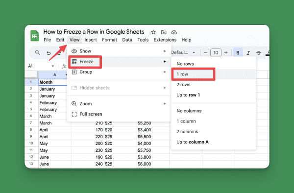
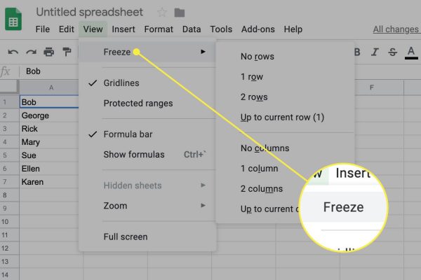
2. Navigate to the View Menu: Click on the “View” tab in the top menu bar.

3. Freeze Option: Select “Freeze” from the drop-down menu. You’ll see options to freeze either “Up to row 1” or “Up to current row” (depending on your selection in step 1).

4. Choose Your Freeze Level: Click on “Up to row 1” to freeze the first row (or any row you selected in step 1). This will lock that row in place as you scroll down the sheet.

Method 2: Using the Split Pane Feature

1. Click and Drag the Split Pane Line: Locate the grey horizontal line between the row numbers and column letters. Click and hold this line, then drag it down to the row where you want the freeze to occur. Let go of the line when you’ve reached your desired row.

Everything Stays Put: Enjoy Your Frozen Rows!

With either method, the chosen rows will be frozen in place, staying visible at the top of your spreadsheet even as you scroll down. This makes it much easier to keep track of your data and navigate your Google Sheet.

Unfreezing Rows (When You Need a Change)

To unfreeze the rows, simply navigate back to the “View” menu and select “Freeze” again. This time, you’ll see an option to “Unfreeze rows.” Click on that, and your data will scroll freely once more.

Mastering the Freeze: Take Control of Your Spreadsheets

By effectively using the freeze function, you can transform your Google Sheets experience. Keep those essential headers and data points in sight, and navigate your spreadsheets with ease. So next time you’re drowning in data, remember, a simple freeze can make all the difference!